Introduction

When I learned about iterated function systems, I became very interested in them what can be done with them. Despite not having gone over the subject of 3D iterated function systems explicitly, there was no reason why any of the subject matter learned in class could not be applied in 3D. It seemed like there would be non-trivial problems to solve in converting some of the classic 2D fractals to 3D, and hence I thought this would make a good topic for my final project.

This paper describes the nuisances of adapting a IFS rendering algorithm to 3D. A companion program was created called IFS3d which was made to accompany this paper and show some of the results. IFS3d's use is explained in the next section. We will explore the process of adapting many famous 2D iterated function systems (such as Sierpinski's Gasket) to their 3D counterparts.

How to use IFS3d

IFS3d is a program created to accompany this paper, so that some of the elements of this paper may be tested and demonstrated. It is written in C++ and the source code is available. IFS3d uses SDL and OpenGL to setup and render to the graphic display.

IFS3d is executed from the command line. IFS3d take one parameter, the name of the input file to open and read the IFS to render from. For example you may type IFS3d Gasket3D.ifs to start IFS3d displaying a 3d version of Sierpinski's Gasket.

When IFS3d is opened, it will initialize with the camera looking at the center of the fractal. You can control the position of the camera in various ways through the mouse. When the left mouse button is pressed, mouse movements will result in rotations of the camera. If both the left and right mouse buttons are pressed, vertical mouse movements will be interpreted as zooming in and out of the fractal. Pressing the ESC key will quit the program.

When the number key 1 is pressed, the camera will be set to a perspective projection (default). The camera can be set to an orthographic projection by pressing 2. Orthographic mode may be helpful in examining the 2d appearance of a 3d fractal from some angle. Finally if 3 is pressed, the z values of the points will be interpreted as time values, and the remaining x and y coordinates are plotted as if we were rendering a 2d fractal. When in the mode resulting from hitting 3, z values will continuously move from 0 to 1 over 5 seconds, and then repeat.

One may notice 8 red dots on the display when moving the camera around. The dots highlight the corners of the unit box (0,0,0) - (1,1,1). They are displayed to give a sense of scale. Notice how fractals such as Sierpinski's Gasket always stay within the box.

IFS File Format

The IFS file is simply a text file. It is parsed as follows:

<Name of IFS>
iterations <IterationCount>
functionCount <NumberOfFunctions>
VariationName Weight <a b c d e f g h j k l m>
- ... (<NumberOfFunctions> times)

All italics text in the above template mean user specified values. All non-italics text indicates a string literal that must be typed exactly that way.

Name of IFS is simply any string terminated by a new line character which will be used as the title of your IFS. IterationCount is the number of points that will be iterated (and plotted). The higher this number is, the denser (and more accurate) your IFS' fixed point will appear. NumberOfFunctions is the number of functions that are part of the system.

The next lines (and there will be NumberOfFunctions of them), define the functions that make up the IFS. VariationName can be either linear, sinusoidal or spherical. Choosing linear will give you a standard affine transformation. Choosing either sinusoidal or spherical will apply an extra mapping to the points after they have been multiplied by the affine matrix. This feature is an afterthought and not supported very well, so most examples provided simply use linear. Weight is the weight that will be given to the current function when the IFS plotting algorithm needs to choose a random function in the system. The number is relative to the total weights of all functions. The following numbers represent entries in a 4x4 affine matrix as follows:

a b c d

e f g h

j k l m

0 0 0 1

The best way to learn the IFS file format is of course to look at any of the provided examples.

Difference between viewing fractals in 3D instead of 2D

Although most aspects of viewing fractals in 2D are unchanged when viewing them in 3D, there are still some subtle differences. In 2D your perspective is normally fixed, in that the resolution of the screen doesn't change, and so most algorithms simply snap every point produced to the closest pixel on the screen. This is not necessary (and even undesirable) in 3D, since the camera may zoom in or out or rotate, all of which would look bad if every point was snapped to a grid.

Points then, are instead stored exactly as they are generated. The points are generated once at the beginning of IFS3d execution and then they are simply re-rendered every frame, transformed by the camera transform. Since the points are drawn in their exact locations, it is possible to zoom in on one area of the fractal until you can see individual points, and then zoom in farther right in to one single point.

Although obvious, it's worth noting that no changes need to be made to the point generating algorithm, as it works for all dimensions.

Adapting 2D Fractals to 3D

This section will analyze a number of different popular 2D fractals, and how one would go about importing them in to a 3D environment. It should be noted that all 2D fractals can be created within a 3D environment by simply j = k = l = m = c = g = 0, and treating the remaining values a, b, d, e, f, and h as you would in a standard 2D affine transformation.

Sierpinski's Gasket

Sierpinski's Gasket is the popular fractal of a triangle with a triangle cut out of it (creating 3 sub-triangles of which this step is applied recursively).

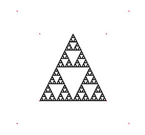Figure 1: Sierpinski's Gasket in 2D (Gasket2D.ifs)

Sierpinski's Gasket can be created by using 3 affine functions:

0.5  0    0    0

0    0.5  0    0

0    0    0    0

0    0    0    1


0.5  0    0    0.5

0    0.5  0    0

0    0    0    0

0    0    0    1


0.5  0    0    0.25

0    0.5  0    0.5

0    0    0    0

0    0    0    1

Which maps the unit cube in to 3 unit squares (with z = 0, this is 2d) in a triangle formation.

One would imagine that a 3D version of Sierpinski's Gasket might have the form of a pyramid instead of a triangle (or an extruded triangle). Similar to how Sierpinski's Gasket was constructed in 2D, we may visualize 4 boxes lying on the ground, with 1 box sitting on the middle of all of these. One may visualize that if we subdivide these 5 boxes one more time, we will have the top pyramid using as a base the bottom 4 pyramids, and we realize that this solution may be feasible. We test our solution by entering following matrices in to IFS3d (one function for every box, positioned in each different location). Since we are dealing with 3 dimensions now, we must not project away the z values to 0. The matrices follow:

0.5  0    0    0

0    0.5  0    0

0    0    0.5  0

0    0    0    1


0.5  0    0    0

0    0.5  0    0

0    0    0.5  0.5

0    0    0    1


0.5  0    0    0.5

0    0.5  0    0

0    0    0.5  0.5

0    0    0    1


0.5  0    0    0

0    0.5  0    0

0    0    0.5  0.5

0    0    0    1


0.5  0    0    0.25

0    0.5  0    0.5

0    0    0.5  0.25

0    0    0    1

And indeed, this gives us a 3D version of Sierpinski's Gasket.

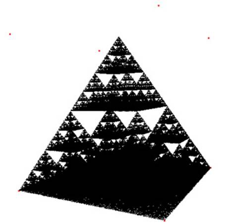Figure 2: Sierpinski's Gasket in 3D (Gasket3D.ifs)

The Cantor set

One might define a 3D Cantor Set to be {x,y,z | x belongs to C, y belongs to C, z belongs to C}. Under this definition we can see that the set is contained within 8 cubes of side length 1/3, each in one corner of the unit cube. Under this reasoning we may proceed in the same fashion as we did for Sierpinski's Gasket (by shrinking the unit cube by 1/3 and then transforming it to a corner of the unit cube) to obtain an 8 function system which converges to the Cantor Set in 3D.

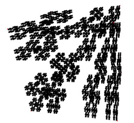Figure 3: Cantor Set in 3D (Cantor3D.ifs)

The Fern

The fern is a much trickier IFS to convert to 3D, partly because it's a trickier IFS than the previous systems even in 2D. The 2D fern can of course be displayed in a 3D environment, but one might expect to see the branches popping out in a true 3D version of it (so perhaps it will be more of a bush than a fern).

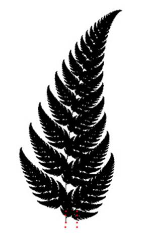Figure 4: Fern in 2D (2DFern.ifs)

The fern is composed of four functions. One of them is the stem, and it projects all points on to the Y axis to form a straight line. Two functions are used to place leaves on the left and right. These are achieved by transforming up in the Y direction, scaling down and rotating around the Z axis by roughly 30 degrees. The last function represents the rest of the fern, and transforms it by shrinking it slightly, rotating it around the Z axis slightly, and transforming up in the Y direction a bit. The system can be examined by looking at the example Fern2D.ifs.

A first attempt at converting the fern to 3D might be to modify the function responsible for drawing the rest of the fern so that it includes a rotation around the Y axis (as well as its rotation around the Z axis). This may be accomplished by taking the original matrix, F, and obtaining the new matrix, F' as follows:

F' = F * RotY

where RotY is a matrix representing a rotation around the Y axis. A rotation around the Y axis can be described as:

cos(ANGLE)     0         sin(ANGLE)     0

0              1         0              0

-sin(ANGLE)    0         cos(ANGLE)     0

0              0         0              1

where ANGLE is the angle of the rotation. Entering this new system (Fern3D.ifs) we do indeed obtain a 3d fern, but it is very bushy and difficult to see what is happening.

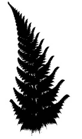Figure 5: Fern in 3D, first attempt (3DFern.ifs)

Certainly there must be a more visually concise system. Much of the incoherency of the above image is caused from the leaves also being bushy (and so the leaves of the leaves, and etc�). We need to find a way to keep the 3d rotations while restricting the rotations within the leaves. One way to accomplish this would be to, for each leaf, project our fern to the XY-plane, and THEN rotate it. This process is similar to how the stem is constructed, except instead of projecting to an axis, we are projecting to a plane. A matrix that projects to the XY-plane is given as:

And so, if we have the original transformations for the two leaves, T1 and T2, we can form T1' and T2' as follows:

T1' = T1 * Proj

T2' = T2 * Proj

Where Proj is the projection matrix defined above. Running the new system through IFS3d gives a much prettier and coherent 3D version of the fern (ReFlattened3DFern.ifs)

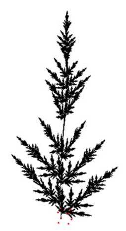Figure 6: Fern in 3D with flattened leaves (ReFlattened3DFern.ifs)

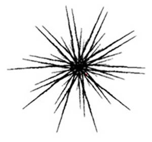Figure 7: Flattened leaf fern viewed from above

The top down view makes it obvious how flat the leaves really are though (even though this is not obvious from most other angles), but perhaps we can fix this as well by having the leaves make a slight rotation around their Y-axis after they have been projected. This can be accomplished by forming a rotation matrix around the Y-axis, RotY, and instead construct T1' and T2' as follows:

T1' = T1 * RotY * Proj

T2' = T2 * RotY * Proj

Since the projection is the last matrix in the matrix multiplication chain, it will be a plied before the rotation around the Y-axis, so the rotation will not be lost to the projection.

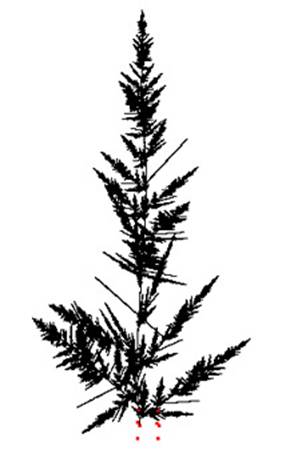Figure 8: Fern with leaves rotated around Y (Final3DFern.ifs)

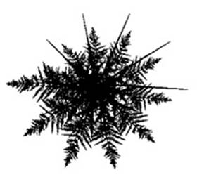Figure 9: Final version of 3D fern viewed from above

The final fern IFS is given in Final3DFern.ifs.

Conclusion

Although all of the concepts of iterated function systems remain the same, regardless of how many dimensions we're operating in, there are still some subtle practical considerations to take in to account when moving from 2D fractals to 3D fractals. The algorithm itself, for example, cannot assume anymore that we are operating on a grid, and so we must store all exact values for points.

Clearly the set of 3D fractals contains the set of 2D fractals (we can always project to 0 on the z-axis) and with examples like the 3D fern, we see that there are many more complicated iterated function systems that cannot be generated in 2D. Given the proper knowledge of how matrix transformations can be applied to functions in IFS to produce intended results, we can sculpt many different shapes in 3D simply by plotting points.

Andrew Top

3D Iterated Function Systems

References

Gulick, D., Encounters with Chaos, Pp. 1-320, ©McGraw-Hill Education, 1992.